1 Introduction

Contains both results from hambiNMR experiment and also a test of using “Just A Plate” cleanup method during library preparation.

2 Setup

2.1 Libraries

library(tidyverse)
library(here)
library(fs)
library(archive)
library(scales)
source(here::here("R", "utils_generic.R"))

2.2 Global variables

data_raw <- here::here("_data_raw", "20240513_BTK_illumina_v3")
data <- here::here("data", "20240513_BTK_illumina_v3")
amplicontar <- here::here(data_raw, "rbec_output.tar.gz")

# make processed data directory if it doesn't exist
fs::dir_create(data)

# create temporary location to decompress
tmpdir <- fs::file_temp()

2.3 Data

NOTE! We have commented out the locus H1279_03957 from HAMBI_1279 because we know HAMBI_1279 is not present in this experiment and that any reads mapping to 1279 come from crosstalk between the 23 species control samples and the experimental samples. HAMBI_1279 shares an exact copy of the V3 region of the 16S gene with HAMBI_1299.

tax_locus_copynum <- tibble::tribble(
     ~strainID, ~rRNA16S_cn, ~rRNA16S_locus,             ~genus,        ~species,
  "HAMBI_0006",          7L,  "H0006_04757",      "Pseudomonas",        "putida",
  "HAMBI_0097",          7L,  "H0097_00044",    "Acinetobacter",     "johnsonii",
  "HAMBI_0097",          7L,  "H0097_02759",    "Acinetobacter",     "johnsonii",
  "HAMBI_0097",          7L,  "H0097_01762",    "Acinetobacter",     "johnsonii",
  "HAMBI_0105",          4L,  "H0105_02306",    "Agrobacterium",   "tumefaciens",
  "HAMBI_0262",          3L,  "H0262_00030",    "Brevundimonas",       "bullata",
  "HAMBI_0403",          9L,  "H0403_00517",        "Comamonas",  "testosteroni",
  "HAMBI_0403",          9L,  "H0403_00522",        "Comamonas",  "testosteroni",
  "HAMBI_1279",          7L,  "H1279_03627",           "Hafnia",         "alvei",
  "HAMBI_1279",          7L,  "H1279_00125",           "Hafnia",         "alvei",
  #"HAMBI_1279",          7L,  "H1279_03957",           "Hafnia",         "alvei",
  "HAMBI_1287",          7L,  "H1287_03997",      "Citrobacter",        "koseri",
  "HAMBI_1287",          7L,  "H1287_03402",      "Citrobacter",        "koseri",
  "HAMBI_1292",          7L,  "H1292_03239",       "Morganella",      "morganii",
  "HAMBI_1299",          8L,  "H1299_04293",         "Kluyvera",    "intermedia",
  "HAMBI_1299",          8L,  "H1299_01283",         "Kluyvera",    "intermedia",
  "HAMBI_1299",          8L,  "H1279_03957",         "Kluyvera",    "intermedia",
  "HAMBI_1842",          4L,  "H1842_01650",      "Sphingobium",    "yanoikuyae",
  "HAMBI_1896",          4L,  "H1896_00963", "Sphingobacterium",  "spiritivorum",
  "HAMBI_1972",         10L,  "H1972_00343",        "Aeromonas",        "caviae",
  "HAMBI_1972",         10L,  "H1972_03531",        "Aeromonas",        "caviae",
  "HAMBI_1977",          5L,  "H1977_00118",      "Pseudomonas",  "chlororaphis",
  "HAMBI_1988",          5L,  "H1988_05160",     "Chitinophaga",        "sancti",
  "HAMBI_1988",          5L,  "H1988_05152",     "Chitinophaga",        "sancti",
  "HAMBI_1988",          5L,  "H1988_05165",     "Chitinophaga",        "sancti",
  "HAMBI_2159",          4L,  "H2159_01406",        "Trinickia",   "caryophylli",
  "HAMBI_2159",          4L,  "H2159_05851",        "Trinickia",   "caryophylli",
  "HAMBI_2160",          3L,  "H2160_00530",       "Bordetella",         "avium",
  "HAMBI_2164",          5L,  "H2164_03337",      "Cupriavidus",    "oxalaticus",
  "HAMBI_2443",          3L,  "H2443_00128",       "Paracoccus", "denitrificans",
  "HAMBI_2494",          4L,  "H2494_03389", "Paraburkholderia",   "kururiensis",
  "HAMBI_2659",          4L,  "H2659_00367", "Stenotrophomonas",   "maltophilia",
  "HAMBI_2792",          4L,  "H2792_00549",        "Moraxella",         "canis",
  "HAMBI_3031",          2L,  "H3031_00830",         "Niabella",  "yanshanensis",
  "HAMBI_3237",          6L,  "H3237_00875",       "Microvirga",   "lotononidis",
  "HAMBI_1923",          6L,  "H1923_00876",   "Flavobacterium",      "odoratum"
  )

2.4 Functions

# this function 
normalize_by_copy <- function(.data, tlc = tax_locus_copynum){
  .data %>% 
    # join with the copy number data frame. We join by the locus tag so this will add H1279_03957 to HAMBI_1299
    dplyr::left_join(tlc, by = join_by(rRNA16S_locus)) %>%
    # get total number of mapping reads per species. This aggregates all the difference ASVs per species
    dplyr::summarize(count = sum(count), .by = c(sample, strainID, rRNA16S_cn)) %>% 
    # group by sample
    dplyr::group_by(sample) %>% 
    # calculate a corrected count which is simply the count divided by copy num for each species
    # dividide by the sum of count divided by copy num for whole sample multiplied by the total
    # number of mapped reads per sample
    dplyr::mutate(count_correct = round(sum(count)*(count/rRNA16S_cn)/sum(count/rRNA16S_cn))) %>%  
    dplyr::ungroup() %>% 
    dplyr::select(sample, strainID, count, count_correct)
  }

# this function replaces missing species counts with zero
completecombos <- function(.data, tlc = tax_locus_copynum, countname = count, remove1923 = TRUE){
 
  # get unique strainIDs
  strainID <- unique(tlc$strainID)
  # table for assigning genus and species names. Doesn't matter if 1923 is there or not
  # because it is filter joined later
  tax <- dplyr::distinct(dplyr::select(tlc, strainID, genus, species))
  if (remove1923) {
    # get unique strainIDs but exclude 1923 if remove1923 is true
    strainID <- strainID[strainID != "HAMBI_1923"]
  }
  
  dplyr::bind_rows(tibble::tibble(strainID = strainID, sample = "dummy"), .data) %>% 
    dplyr::mutate( "{{ countname }}" := dplyr::if_else(sample == "dummy", 1, {{ countname }})) %>% 
    tidyr::complete(sample, strainID) %>% 
    dplyr::filter(sample != "dummy") %>% 
    dplyr::mutate( "{{ countname }}" := dplyr::if_else(is.na({{ countname }}), 0, {{ countname }})) %>% 
    tidyr::replace_na(list(count_correct = 0)) %>% 
    dplyr::left_join(dplyr::distinct(dplyr::select(tlc, strainID, genus, species))) %>% 
    dplyr::relocate(genus, species, .after = strainID)
}

3 Read metadata

mddf <- readr::read_tsv(here::here(data_raw, "20240513_BTK_illumina_v3_metadata.tsv"))

Rows: 414 Columns: 6
── Column specification ────────────────────────────────────────────────────────
Delimiter: "\t"
chr (6): sample, exp_type, cleanup, exp_replicate, growth_phase, tech_replicate

ℹ Use `spec()` to retrieve the full column specification for this data.
ℹ Specify the column types or set `show_col_types = FALSE` to quiet this message.

4 Read Rbec raw counts tables

4.1 Untar Rbec output tarball

archive::archive_extract(
  amplicontar,
  dir = tmpdir,
  files = NULL,
  options = character(),
  strip_components = 0L
)

4.2 Setup directory structure

tabdir <- here::here(tmpdir, "rbec_output")
samppaths <- fs::dir_ls(tabdir)
sampnames <- path_split(samppaths) %>% 
  map_chr(dplyr::last)

4.3 Read

straintabs <- paste0(samppaths, "/strain_table.txt") %>% 
  set_names(sampnames) %>% 
  map_df(
  read_tsv,
  skip = 1,
  col_names = c("rRNA16S_locus","count"),
  show_col_types = FALSE, 
  .id = "sample")

5 Format

Normalize counts by 16S copy number

straintabs_norm <- normalize_by_copy(straintabs)

Complete all combinations of 23 species

straintabs_norm_fmt <- completecombos(straintabs_norm, tlc = tax_locus_copynum, countname = count, remove1923 = TRUE)

Joining with `by = join_by(strainID)`

finaltable <- left_join(straintabs_norm_fmt, mddf)

Joining with `by = join_by(sample)`

6 Analysis

6.1 Negative controls

Note: labels for positive controls and negative controls for plates 1+2 were accidentally swapped on the plates. This has been corrected in post processing

First, we’ll check whether the experimental and plate negative controls look good

finaltable %>% 
  filter(str_detect(exp_type, "^neg|pos")) %>% 
  summarize(tot = sum(count_correct), .by = c("sample", "exp_type", "cleanup", "exp_replicate", "growth_phase"))

This looks great. In all cases very few reads are coming off the negative controls. This means it is safe to assume there was no contamination during the library preps. More importantly it looks like the main experiment was clean because we see no growth/contamination in the R2A media blanks.

6.2 Positive controls

finaltable %>% 
  filter(str_detect(exp_type, "^pos|^neg")) %>%
  mutate(total_pos_controls = n_distinct(sample)) %>% 
  group_by(sample) %>% 
  mutate(n_sp_detected = sum(count > 0)) %>% 
  distinct(sample, n_sp_detected, total_pos_controls)

This is also good - we detect all 23 species in the positive controls on each plate (again considering that the Pos/Neg replicates 1+2 are switched)

6.3 Pairwise samples

First off important information: there are only 16 species in these experiments not all 23. These species were selected as the top 16 most abundant from the YSK experiment

sps <- c("HAMBI_0006", "HAMBI_0105", "HAMBI_0403", "HAMBI_1287",
         "HAMBI_1292", "HAMBI_1299", "HAMBI_1842", "HAMBI_1896", 
         "HAMBI_1972", "HAMBI_1977", "HAMBI_2160", "HAMBI_2164", 
         "HAMBI_2443", "HAMBI_2659", "HAMBI_3031", "HAMBI_3237")

Here we need to account for the fact that HAMBI_1279 and HAMBI_1299 share one identical copy of the 16S rRNA V3 region. In the current pipeline reads mapping to this shared amplicon are distributed equally to the two species. However, we will need to redistribute all reads mapping to HAMBI_1279 to HAMBI_1299 since 1279 wasn’t included in the experiment.

pairs <- finaltable %>%
  filter(exp_type == "pair") %>% 
  tidyr::separate(sample, into = c("sp1", "sp2", "x", "y"), sep = "\\+|_", remove = FALSE) %>% 
  mutate(sp1 = paste0("HAMBI_", sp1),
         sp2 = paste0("HAMBI_", sp2)) %>% 
  dplyr::select(-x, -y) %>% 
  group_by(sample) %>% 
  mutate(f = count_correct/sum(count_correct)) %>% 
  ungroup()

Warning: Expected 4 pieces. Missing pieces filled with `NA` in 5520 rows [1, 2, 3, 4, 5,
6, 7, 8, 9, 10, 11, 12, 13, 14, 15, 16, 17, 18, 19, 20, ...].

Here we focus on samples with species that should not be there. We exclude species that were inoculated and plot the distribution of percentages of those species

Figure 1: Frequency distribution of each species in pairwise samples where it should not occur from the Norgen-normalized samples. The 1% mark (commonly accepted as an acceptable Illumina cross-talk standard) is demarcated with a dashed line.

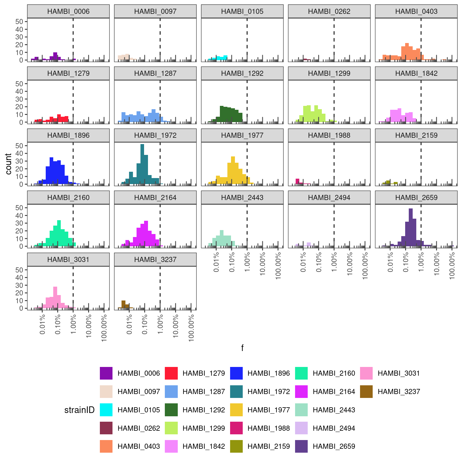
Here we can see that all species are below the 1% threshold which is more or less what you can expect when you are multiplexing libraries on an Illumina platform. Values greater than 1% are indicative of a different problem. So this is good.

Quick look at how the “Just Another Plate” cleanup and normalization approach worked.

Figure 2: Frequency distribution of each species in pairwise samples where it should not occur from the “Just Another Plate” normalized samples. The 1% mark (commonly accepted as an acceptable Illumina cross-talk standard) is demarcated with a dashed line.

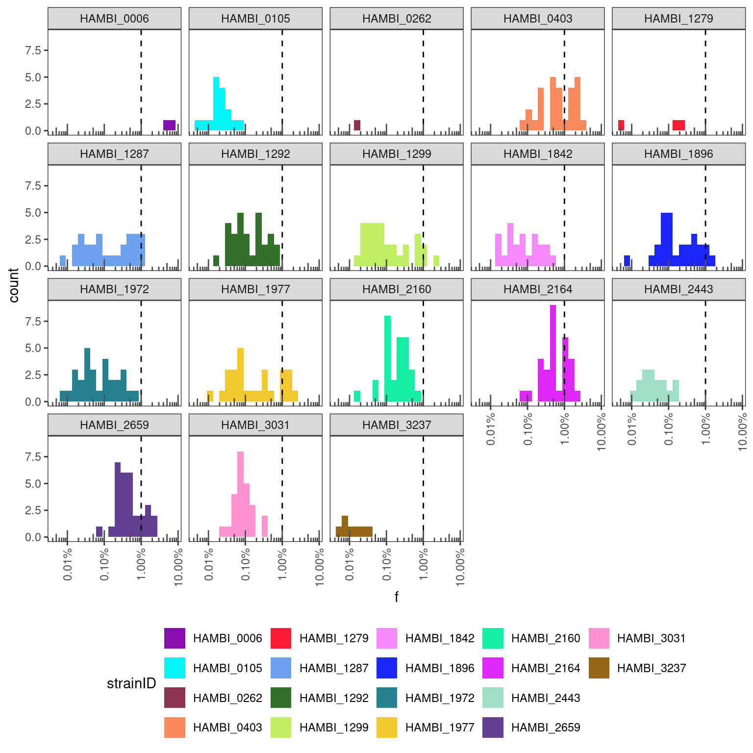
This also looks pretty ok I think… Perhaps the JAP is a bit worse at cleaning up and so there is some slightly higher cross talk from some species. For example, it looks like HAMBI_2659 is hitting ~2% crosstalk in some instances. There are also fewer samples that were tested with JAP so counts are lower and the distributions will be more noisy. Still most are well under 1%.

Here we’ll focus on any problematic samples that have over 10% of a species that shouldn’t be there.

contaminated_samples <- pairs %>% 
  filter(cleanup == "norgen") %>% 
  mutate(contam = if_else(sp1 != strainID & sp2 != strainID, 1, 0)) %>% 
  group_by(sample) %>% 
  filter(contam == 1) %>% 
  filter(f >= 0.1) %>% 
  ungroup()

contaminated_samples

There are two samples where there may have just been some random droplet that contaminated them.

1292+2443_r2 has 80% HAMBI_2659
1842+1896_r2 has 30% HAMBI_0403

pairs_final <- pairs %>% 
  filter(cleanup == "norgen") %>% 
  filter(sample %nin% contaminated_samples$sample) %>%
  group_by(sample) %>% 
  mutate(tot = sum(count_correct)) %>% 
  ungroup() %>% 
  filter(sp1 == strainID | sp2 == strainID) %>% 
  select(sample, strainID, exp_replicate, count_correct) %>% 
  group_by(sample) %>% 
  mutate(f = round(count_correct/sum(count_correct), 3))

write_tsv(pairs_final, here::here(data, "pairs_counts.tsv"))

6.4 LOO communities

LOO_communities <- finaltable %>% 
  filter(str_detect(exp_type, "loo")) %>%
  tidyr::separate(sample, into = c("x", "sp1", "y", "z"), sep = "-|_", remove = FALSE) %>% 
  mutate(loo_sp = paste0("HAMBI_", sp1)) %>% 
  dplyr::select(-x, -y, -z, -sp1) %>% 
  relocate(sample, loo_sp) %>% 
  group_by(sample) %>% 
  mutate(f = count_correct/sum(count_correct)) %>% 
  ungroup()

Warning: Expected 4 pieces. Additional pieces discarded in 1104 rows [1, 2, 3, 4, 5, 6,
7, 8, 9, 10, 11, 12, 13, 14, 15, 16, 17, 18, 19, 20, ...].

Warning: Expected 4 pieces. Missing pieces filled with `NA` in 1472 rows [70, 71, 72,
73, 74, 75, 76, 77, 78, 79, 80, 81, 82, 83, 84, 85, 86, 87, 88, 89, ...].

Have a look at contaminant species - how bad is it? A: pretty good!

LOO_communities %>% 
  filter(strainID %nin% sps) %>% 
  filter(f > 0) %>% 
  summarize(max(f), min(f), mean(f), median(f), .by = c(growth_phase, strainID))

So cross talk from for example the positive controls is very minimal (which is to be expected since there are so few positive control samples).

But now we should check how many LOO samples have the species that was supposed to be “LOO-ed” and at what frequency.

LOO_communities %>%
  filter(cleanup == "norgen") %>% 
  # from each sample exclude the species that are supposed to be there
  # and focus only on contaminants
  filter(loo_sp == strainID ) %>% 
  summarize(max(f), min(f), mean(f), median(f), .by = c(loo_sp, growth_phase))

Ok again this looks really good. All “LOO-ed” species are properly missing from the corresponding samples both in the inoculate and the post_growth phases.

LOO_communities_final <- LOO_communities %>% 
  filter(cleanup == "norgen") %>% 
  # remove LOO'ed species that should not be there
  filter(loo_sp != strainID ) %>%
  filter(strainID %in% sps) %>% 
  dplyr::select(-count, -f, -exp_type, -cleanup) %>% 
  group_by(sample) %>%
  mutate(f = round(count_correct/sum(count_correct), 3),
        tot = sum(count_correct)) %>%
  ungroup() %>%
  relocate(tot, f, .after = count_correct)

write_tsv(LOO_communities_final, here::here(data, "loo_communities_counts.tsv"))

6.5 Full communities

Checking on species that shouldn’t be there…

finaltable %>% 
  filter(str_detect(exp_type, "full_community")) %>%
  filter(strainID %nin% sps) %>% 
  filter(count_correct > 0)

So the only species that shouldn’t be in those samples is HAMBI_1279 but it is at very low concentrations

full_communities_final <- finaltable %>% 
  filter(str_detect(exp_type, "full_community")) %>%
  filter(cleanup == "norgen") %>% 
  filter(strainID %in% sps) %>% 
  dplyr::select(-count, -exp_type, -cleanup) %>% 
  group_by(sample) %>% 
  mutate(f = round(count_correct/sum(count_correct), 3),
         tot = sum(count_correct)) %>% 
  ungroup() %>% 
  relocate(tot, f, .after = count_correct)

write_tsv(full_communities_final, here::here(data, "full_communities_counts.tsv"))

7 Clean up

# remove decompressed coverage directory from temp location
fs::dir_delete(tmpdir)